Finite difference
A finite difference is a mathematical expression of the form
$$f(x_0)-f(x_1)$$
If a finite difference is divided by \((x_0-x_1)\), one gets a difference quotient:
$$\frac{f(x_0)-f(x_1)}{x_0-x_1}$$
Approximation of Derivative
Taylor series
Consider the Taylor series expansion of function \(f(x)\):
$$\begin{align*} f(x) &= \sum_{n=0}^{\infty} \frac{f^{(n)}(x_0)}{n!} (x - x_0)^n = \\ &= f(x_0) + f'(x_0)(x-x_0) + \frac{f''(x_0)}{2!}(x-x_0)^2 + \frac{f'''(x_0)}{3!}(x-x_0)^3 + \cdots \end{align*}$$
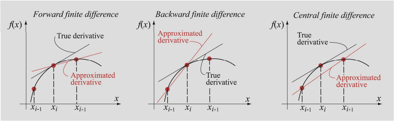
Forward difference
Assuming \(x=x_0+h\), where \(h\) represents a small increment from \(x_0\) we obtain:
$$\begin{align*} & f(x_0 + h) = f(x_0) + f'(x_0)h + \frac{f^{(2)}(x_0)}{2!}h^2 + \frac{f^{(3)}(x_0)}{3!}h^3 + \frac{f^{(4)} (x_0)}{4!}h^4 +\cdots & \text{(1)} \end{align*}$$
Rearranging the terms, we obtain:
$$ \frac{f(x_0 + h)-f(x_0)}{h} = f'(x_0) + \frac{f^{(2)}(x_0)}{2!}h + \frac{f^{(3)}(x_0)}{3!}h^2 + \frac{f^{(4)} (x_0)}{4!}h^3 +\cdots$$
That is to say:
$$ \frac{f(x_0 + h)-f(x_0)}{h} = f'(x_0) + O(h)$$
Backward difference
Assuming \(x=x_0-h\), where \(h\) represents a small increment from \(x_0\) we obtain:
$$\begin{align*} & f(x_0 - h) = f(x_0) - f'(x_0)h + \frac{f^{(2)}(x_0)}{2!}h^2 - \frac{f^{(3)}(x_0)}{3!}h^3 + \frac{f^{(4)} (x_0)}{4!}h^4 -\cdots & \text{(2)} \end{align*}$$
Rearranging the terms, we obtain:
$$ \frac{f(x_0)-f(x_0 - h)}{h} = f'(x_0) - \frac{f^{(2)}(x_0)}{2!}h + \frac{f^{(3)}(x_0)}{3!}h^2 - \frac{f^{(4)} (x_0)}{4!}h^3 +\cdots$$
That is to say:
$$ \frac{f(x_0)-f(x_0 - h)}{h} = f'(x_0) + O(h)$$
Central difference
Finally, the central difference is given by:
$$ \frac{f(x_0+h)-f(x_0-h)}{2h}$$
whose numerator is given by the difference \((1)-(2)\). In this way we obtain:
$$ \frac{f(x_0+h)-f(x_0-h)}{2h}= f'(x_0) + \frac{f^{(3)}(x_0)}{3!}h^2 + \frac{f^{(5)}(x_0)}{5!}h^4 +\cdots$$
That is to say:
$$ \frac{f(x_0+h)-f(x_0-h)}{2h}= f'(x_0) + O(h^2)$$
Second derivative - Three-point Central Difference Formula
If we add (1) and (2) together we obtain:
$$ f(x_0 + h) + f(x_0 - h) = 2f(x_0) + 2\frac{f^{(2)}(x_0)}{2!}h^2 + 2\frac{f^{(4)}(x_0)}{4!}h^4 + \cdots$$
If we solve it for \(f^{(2)}(x_0)\) we obtain:
$$ f^{(2)}(x_0) = \frac{f(x_0 + h) - 2f(x_0) + f(x_0 - h)}{h^2} + O(h^2)$$
Example
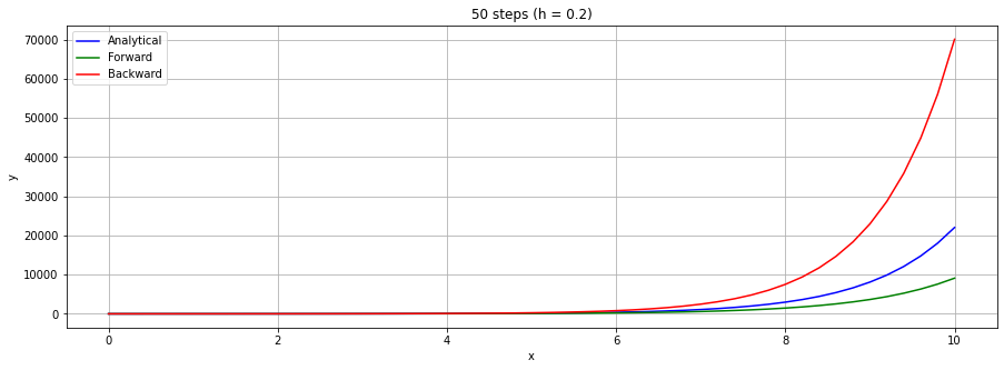
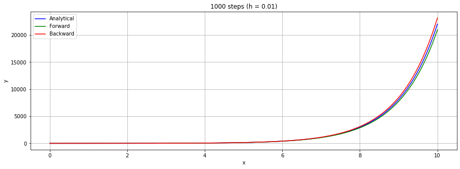
Utilizing the backward and forward difference, we numerically solve the equation $$y'=y$$ with the initial condition y(0)=0. We know that the analytical solution is \(y(x)=e^x\), but let's comapare it whith the numerical solutions.
First of all we set \(x_{i+1}=x_i+h\) and \(y(x_i)=y_i\)
- Using Forward difference we have: $$y_i=y_{i-1}(h+1)$$
- Using Backward difference we have: $$ y_i=\frac{y_{i-1}}{(1-h)}$$
Python Code
    import numpy as np
    import matplotlib.pyplot as plt
    import math

    end = 10.0  # final x
    n = 1000  # iterations
    h = end / n  # integration step

    y_0 = 1  # start condition

    # Lists
    for_values = [y_0]
    back_values = [y_0]
    analitical_values = [y_0]
    h_values = [0]

    for i in range(1, n + 1):
        f_new = for_values[i - 1] * (h + 1)
        b_new = back_values[i - 1] / (1 - h)
        h_new = i * h
        a_new = math.pow(math.e, h_new)

        h_values.append(h_new)
        for_values.append(f_new)
        back_values.append(b_new)
        analitical_values.append(a_new)

    for_values = np.array(for_values)
    back_values = np.array(back_values)
    analitical_values = np.array(analitical_values)
    h_values = np.array(h_values)

    # Plot diagram
    plt.figure(figsize=(15, 5))
    plt.plot(h_values, analitical_values, label='Analytical', color='blue')
    plt.plot(h_values, for_values, label='Forward', color='green')
    plt.plot(h_values, back_values, label='Backward', color='red')

    plt.xlabel('x')
    plt.ylabel('y')
    plt.title('n steps (h = end / n)')
    plt.legend()
    plt.grid(True)
    plt.show()
The outputs
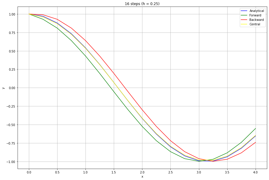
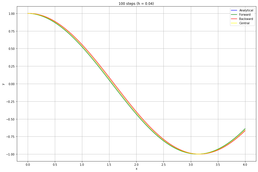
Example
Utilizing the backward, forward and central difference, we numerically find $$y(x)=D(sin(x))$$We know that the analytical solution is \(y(x)=cos(x)\), but let's comapare it whith the numerical solutions.
Python Code
    import numpy as np
    import matplotlib.pyplot as plt
    import math

    end = 4.0  # final x
    n = 100  # iterations
    h = end / n  # integration step

    # Lists
    for_values = [y_0]
    back_values = [y_0]
    central_values = [y_0]
    analitical_values = [y_0]
    h_values = [0]

    for i in range(1, n + 1):
        h_new = h*i
        f_new = ( math.sin(h_new+h) - math.sin(h_new) ) / h
        b_new = ( math.sin(h_new) - math.sin(h_new - h) ) / h
        c_new = ( math.sin(h_new + h) - math.sin(h_new - h)) / (2*h)
        a_new = math.cos(h_new)

        for_values.append(f_new)
        back_values.append(b_new)
        central_values.append(c_new)
        analitical_values.append(a_new)
        h_values.append(h_new)

    for_values = np.array(for_values)
    back_values = np.array(back_values)
    central_values = np.array(central_values)
    analitical_values = np.array(analitical_values)
    h_values = np.array(h_values)

    # Plot diagram
    plt.figure(figsize=(15, 10))
    plt.plot(h_values, analitical_values, label='Analytical', color='blue')
    plt.plot(h_values, for_values, label='Forward', color='green')
    plt.plot(h_values, back_values, label='Backward', color='red')
    plt.plot(h_values, central_values, label='Central', color='yellow')


    plt.xlabel('x')
    plt.ylabel('y')
    plt.title('n steps (h = end / n)')
    plt.legend()
    plt.grid(True)
    plt.show()
The outputs
Appendix - Big O notation
Let \( f \) and \( g \) be two real functions defined in \( (a, b) \setminus \{x_0\} \) whith \(x_0 \in \widetilde{\mathbb{R}}\). We say that \( f = O(g) \) (read as "f is big-O of g") if there exists \( M \in \mathbb{R} \), with \( M \neq 0 \), such that $$ \lim_{x \to x_0} \frac{f(x)}{g(x)} = M $$ Saying that \( f = O(g) \) roughly means that "the function \( f \) behaves more or less the same way as the function \( g \) as \( x \) tends to \( x_0 \)".
Appendix - Little o notation
Let \( f \) and \( g \) be two real functions defined in \( (a, b) \setminus \{x_0\} \) and infinitesimal as \( x \) tends to \( x_0 \in \widetilde{\mathbb{R}}\), that is, $$ \lim_{x \to x_0} f(x) = \lim_{x \to x_0} g(x) = 0 $$ We say that \( f = o(g) \) (read as "f is little-o of g") if $$ \lim_{x \to x_0} \frac{f(x)}{g(x)} = 0 $$ Note that saying \( f = o(g) \) roughly means that "the function \( f \) vanishes more rapidly than the function \( g \) as \( x \) tends to \( x_0 \)".