Lagrangian vs Eulerian Descriptions of Fluid flow
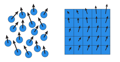
- The Lagrangian specification of the flow field is a way of looking at fluid motion where the observer follows an individual fluid parcel as it moves through space and time.
- The Eulerian specification of the flow field is a way of looking at fluid motion that focuses on specific locations in the space through which the fluid flows as time passes.
Lagrangian vs Eulerian Descriptions of Fluid flow
Velocity Field
Using an Eulerian approach, we divide the 2D space into a grid of side length \( h \). We are employing the MAC (Marker-and-Cell) grid method that simulates fluid flow by periodically updating the velocity field.
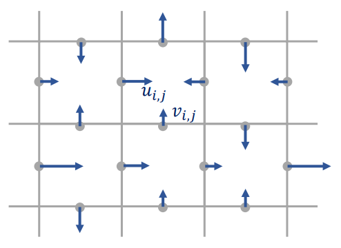
Let's define the vector field \( \mathbf{u} = \begin{bmatrix} u \\ v \end{bmatrix} \) represented as a two-dimensional vector with components \( u \) and \( v \).
Now we apply this vector to the sides of the grid as shown in the figure.
Velocity Field
Therefore, we will assign a scalar value \( s \) to every cell within the grid. Specifically, \( s=0 \) denotes a solid cell, while \( s=1 \) indicates a fluid cell.
                for (var i = 0; i < numX; i++) {
                    for (var j = 0; j < numY; j++) {
                        var s = 1.0;	// fluid
                        if (i == 0 || j == 0 || j == numY-1) {
                            s = 0.0;	// solid
                        }
                        s[i*n + j] = s
                    }
                }
Hypotheses:
- The fluid is assumed to be incompressible: \( \nabla \cdot \mathbf{u} =0 \)
- The fluid is assumed to be non-viscous: \( \mu=0 \)
- The simulation will be conducted in a 2D environment.
Divergence and Incompressibility
Definition: in vector calculus, divergence is a scalar quantity that measures the outward flow rate of a vector field away from a given point within a region of space.
In two-dimensional Cartesian coordinates, the divergence of a continuously differentiable vector field is defined as the scalar-valued function:
$$ \text{div}(\mathbf{u}) = \nabla \cdot \mathbf{u} = \frac{\partial u}{\partial x} + \frac{\partial v}{\partial y} $$
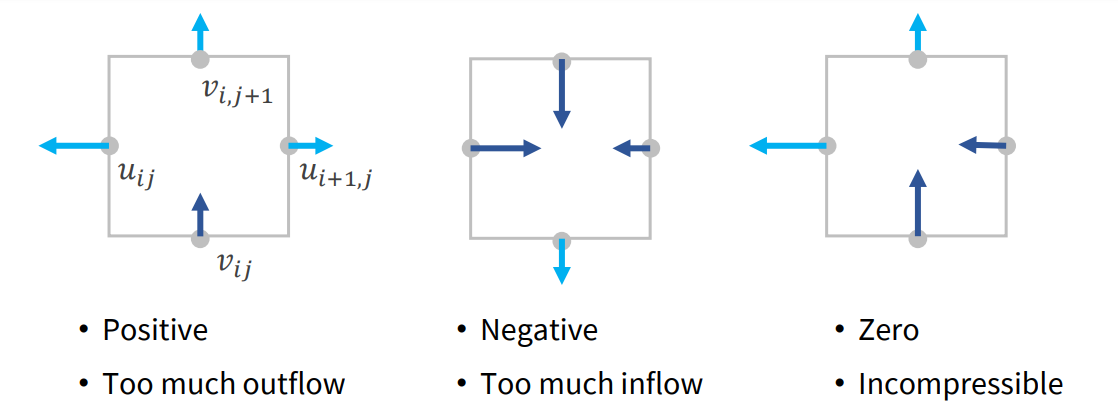
Divergence \( \lesseqgtr 0 \)
To enforce the incompressibility of the fluid, we need to impose \( \nabla \cdot \mathbf{u} =0 \).
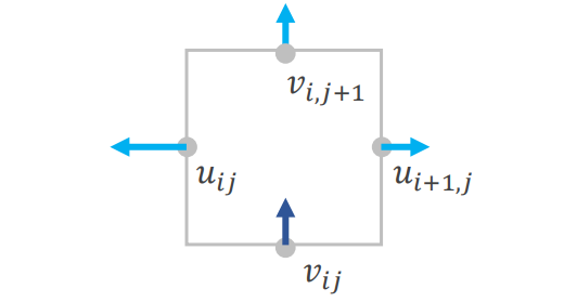
A cell of the grid
To approximate the divergence of a vector field \( \mathbf{u} \) for each \( (i,j) \) cell of the grid we can approximate the partial derivatives in this way:
$$ \frac{\partial u}{\partial x} \approx \frac{u_{i+1,j} - u_{i,j}}{h} $$
$$ \frac{\partial v}{\partial y} \approx \frac{v_{i,j+1} - v_{i,j}}{h} $$
So, the divergence for the \( (i,j) \) cell will be:
$$ \text{div}(\mathbf{u}) \approx \frac{u_{i+1,j} - u_{i,j} + v_{i,j+1} - v_{i,j}}{h} $$
In the simulation we will simplify the divergence calculation by omitting the \( \frac{1}{h} \) factor. This simplification doesn't significantly impact the simulation's accuracy ( \(h\) is equal for each cell)
Therefore, we will multiply the divergence approximation by a parameter \(\omega\) known as the overrelaxation factor. This parameter aids in the convergence of the simulation under the assumption that \( 1 < \omega < 2 \), becouse it enhances the importance of the divergence term.
If we denote the divergence as \(d\) (and the overelaxation parameter as \(\omega\)) in our code it will be represented as:
$$d=\omega \cdot(u_{i+1,j} - u_{i,j} + v_{i,j+1} - v_{i,j})$$
                var d = u[(i+1)*n + j] - u[i*n + j] + v[i*n + j+1] - v[i*n + j];
                d *= overRelaxation;
We have computed the divergence to update velocities at each iteration. During each iteration, the divergence of each cell will be redistributed among adjacent fluid cells.
The number of adjacent fluid cells to each \( (i,j) \) cell is stored in the variable \( ns \)
                var sx0 = s[(i-1)*n + j];
                var sx1 = s[(i+1)*n + j];
                var sy0 = s[i*n + j-1];
                var sy1 = s[i*n + j+1];
                var ns = sx0 + sx1 + sy0 + sy1;
Now, we will now update the velocities as follows:
                u[i*n + j] += sx0 * d / ns ;
                u[(i+1)*n + j] -= sx1 * d / ns;
                v[i*n + j] += sy0 * d / ns;
                v[i*n + j+1] -= sy1 * d / ns;