Stokes' law

Introduction

To analyze the motion of a sphere in a fluid, we require an understanding of three fundamental forces: Stokes' law for viscous drag force ( $ F_d $ ), the buoyant force ( $ F_b $ ) according to Archimedes' principle, and the gravitational force ( $ F_g $ ) or weight of the sphere.

Stokes' Law: Describes the viscous drag force experienced by the sphere due to its motion through the fluid. It is given by $$ F_d = 6 \pi \eta r v $$ where $𝜂$ is the fluid viscosity, $r$ is the radius of the sphere, and $v$ is the velocity of the sphere relative to the fluid.

The force caused by Archimedes' principle on a sphere submerged in a fluid opposes the weight of the displaced fluid. This force can be calculated as $$ F_b= \rho V g = \frac{4}{3}\pi r^{3} \rho g$$ where $\rho$ is the density of the fluid, $V$is the volume of the sphere, and $g$ is the gravitational acceleration.

Gravitational Force (Weight): Represents the downward force due to gravity acting on the sphere. It is given by $$F_g =mg$$ where $m$ is the mass of the sphere and $g$ is the acceleration due to gravity.

Situation

Equation of motion

Putting everything together, we obtain the equation of motion as follows:

$$ m \frac{dv(t)}{dt} = mg -6 \pi \eta r \cdot v(t) - \frac{4}{3}\pi r^{3} \rho g $$

Being a first-order linear nonhomogeneous differential equation, it is possible to solve it. Specifically, assuming $v(0)=0$, the solution is as follows:

$$ v(t) = \frac{3mg-4 \pi r^3 \rho g}{18 \pi \eta r} (1- e^{\frac{-6 \pi \eta r}{m}t})$$

By setting $ \frac{dv(t)}{dt} \approx \frac{v(t+ \Delta t)- v(t)}{\Delta t}$, it is possible to solve it using the finite difference method. Thus, we obtain the following:

$$v(t+ \Delta t) = v(t)+ \frac{\Delta t}{m} (mg -6 \pi \eta r \cdot v(t) - \frac{4}{3}\pi r^{3} \rho g) $$

Simulation

In the following code, we compare the two methods.


    import numpy as np
    import matplotlib.pyplot as plt

    # Parameters
    g = 9.81  # gravitational acceleration (m/s^2)
    eta = 1.2  # fluid viscosity (kg/(m*s))
    r = 0.01  # object radius (m)
    rho_f = 1078  # fluid density (kg/m^3)
    rho_s = 7500  # steel density (kg/m^3)
    m = (4/3) * np.pi * r**3 * rho_s  # object mass (kg)

    # Analytical function
    def v_analytical(t):
        return ((3 * m * g - 4 * np.pi * r**3 * rho_f * g) / (18 * np.pi * eta * r)) * (1 - np.exp(-6 * np.pi * eta * r * t / m))

    # Initial conditions for numerical integration
    v0 = 0.0  # initial velocity (m/s)
    t0 = 0.0  # initial time (s)
    t_end = 3.0  # final time (s)
    n = 1000  # iterations
    dt = t_end / n  # integration time step (s)

    # Lists to store time and velocity values
    t_values = [t0]
    v_values = [v0]

    # Numerical integration loop
    for i in range(1, n+1):
        v_new = v_values[i-1] + (dt / m) * (m * g - 6 * np.pi * eta * r * v_values[i-1] - (4/3) * np.pi * r**3 * rho_f * g)
        t_new = t_values[i-1] + dt
        t_values.append(t_new)
        v_values.append(v_new)

    # Convert lists to numpy arrays
    t_values = np.array(t_values)
    v_values = np.array(v_values)

    # Calculate analytical function values over the time range
    v_analytical_values = v_analytical(t_values)

    # Plot velocity-time diagram
    plt.figure(figsize=(8, 6))
    plt.plot(t_values, v_values, label='Numerical Velocity')
    plt.plot(t_values, v_analytical_values, label='Analytical Velocity', linestyle='--')
    plt.xlabel('Time (s)')
    plt.ylabel('Velocity (m/s)')
    plt.title('Velocity-Time Diagram')
    plt.legend()
    plt.grid(True)
    plt.show()

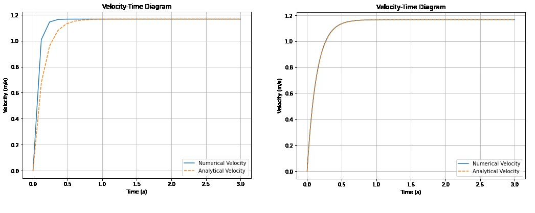
Here are the outputs for $n=25$ and $n=1000$

You can observe that as $n$ increases, the two curves coincide.